the perceptron.

My job doesn’t really allow me to use machine learning or use interesting mathematics in a way that I would like to. As such, to keep both my knowledge fresh and give me something to do, I’ve decided to write what essentially amounts to expositions of important topics in statistical learning.

I find it most logical to start with one of the most basic machine learning algorithms: the perceptron. If you’re reading this, or any other of my “right” type posts (technical stuff) I generally assume basic understanding of linear algebra and probability, though I may elaborate on some of those details if it makes sense in the flow of things.

Anyhoo…

The Perceptron

The perceptron is a classification algorithm that finds a separating hyperplane for data that can be linearly separated into two classes. That is, if the data can be represented as feature vectors \(\mathcal{T} = \{\vec{x}_i \}_{i = 1}^{N} \subseteq \mathbb{R}^n\), and \(y_i = f(x_i) \in \{-1, 1\}\) represents the class of \(\vec{x}_i\), then we are looking for \(\vec{w} \in \mathbb{R}^n\) such that

\[y_i \vec{w}^{T} \vec{x}_i > 0, \forall i\]

Intuitively, we want \(\vec{w}\) so that the sign of \(\vec{w}^{T} \vec{x}_i\) (call this \(\hat{y}_i\)) always matches that of \(y_i\), the actual label of \(\vec{x}_i\), and that this works for all the given feature vectors \(\vec{x}_i\).

The Algorithm

Assume that the dataset is linearly separable; that is,

\[\exists \vec{w}_*, ~~ \forall ~ \vec{x} \in \mathcal{T}, ~~ y_i \vec{w}_*^{T}\vec{x}_i > 0 \qquad (1)\]

The perceptron algorithm finds a \(\vec{w}\) such that \(\forall ~ \vec{x} \in \mathcal{T}, ~~ y_i \vec{w}^{T}\vec{x}_i > 0\) in the following iterative manner:

1. Initialize \(\vec{w}^{(1)} = \vec{0}\), and set iteration \(k\) to be 1.

2. At iteration \(k\), for each vector \(\vec{x}_i \in \mathcal{T}\), compute \(y_i {\vec{w}^{(k)}}^{T} \vec{x}_i\).
   • If all such \(y_i {\vec{w}^{(k)}}^{T} \vec{x}_i > 0\), then \(\vec{w}^{(k)}\) is an appropriate weight vector that separates the classes, and the algorithm terminates.
   • Otherwise, choose some \(\vec{x}^{(k)}\) where \(y^{(k)} {\vec{w}^{(k)}}^{T} \vec{x}^{(k)} \leq 0\), and update \(\vec{w}^{(k + 1)} = \vec{w}^{(k)} + y^{(k)} \vec{x}^{(k)}\).

   Increment iteration counter by 1 (set \(k = k + 1\)).

3. Repeat step 2 until there is a weight vector \(\vec{w}^{(K)}\) such that \(y_i {\vec{w}^{(K)}}^{T} \vec{x}_{i} > 0\), for all \(\vec{x}_i \in \mathcal{T}\)

Intuitively, what this procedure is doing is:

• If I classify a vector correctly, I’m doing good - don’t do anything to the weight vector
• If I misclassify a vector, it means I need to pull the weight vector in the opposite direction it was going from the previous iteration. Then, I need to check everything all over again with the new weight vector.

To prove that this algorithm works, it suffices to show that it terminates; more specifically, we show that \(K\), the number of iterations, is finite.

Proof of Perceptron Algorithm

The idea of the (standard) proof is to show that as \(\vec{w}^{(k)}\) is successively updated through the iterations, the bound for the angle between it and \(\vec{w}_*\) gets closer to 0, and the rate at which this happens increases with \(k\).

Proof.

Consider the weight vector after \(k\) iterations:

\[\vec{w}^{(k)} = \vec{w}^{(k - 1)} + y^{(k - 1)} \vec{x}^{(k - 1)}\]

Taking the dot product of both sides,

\[\begin{align*} \left\lVert \vec{w}^{(k)} \right\rVert^2 &= \left( \vec{w}^{(k - 1)} + y^{(k - 1)} \vec{x}^{(k - 1)} \right) \cdot \left( \vec{w}^{(k - 1)} + y^{(k - 1)} \vec{x}^{(k - 1)} \right) \cr &= {\left\lVert \vec{w}^{(k - 1)} \right\rVert}^2 + 2 y^{(k - 1)} \vec{w}^{(k - 1)} \cdot \vec{x}^{(k - 1)} + \left\rVert y^{(k - 1)} \vec{x}^{(k - 1)} \right\rVert^2 \cr &\leq {\left\lVert \vec{w}^{(k - 1)} \right\rVert}^2 + \left\rVert y^{(k - 1)} \vec{x}^{(k - 1)} \right\rVert^2 \end{align*}\]

as \(2 y^{(k - 1)} \vec{w}^{(k - 1)} \cdot \vec{x}^{(k - 1)} \leq 0\) since \(\vec{w}^{(k - 1)}\) misclassified \(\vec{x}^{(k - 1)}\).

Noting that we can repeat this process downwards for \(k\), we get

\[\begin{align*} \left\lVert \vec{w}^{(k)} \right\rVert^2 &\leq {\left\lVert \vec{w}^{(k - 1)} \right\rVert}^2 + \left\rVert y^{(k - 1)} \vec{x}^{(k - 1)} \right\rVert^2 \cr &\leq {\left\lVert \vec{w}^{(k - 2)} \right\rVert}^2 + \left\rVert y^{(k - 2)} \vec{x}^{(k - 2)} \right\rVert^2 + \left\rVert y^{(k - 1)} \vec{x}^{(k - 1)} \right\rVert^2 \cr &\leq \vdots \cr &\leq {\left\lVert \vec{w}^{(1)} \right\rVert}^2 + \left\rVert y^{(1)} \vec{x}^{(1)} \right\rVert^2 + \ldots + \left\rVert y^{(k - 1)} \vec{x}^{(k - 1)} \right\rVert^2 \cr &\leq \left\rVert y^{(1)} \vec{x}^{(1)} \right\rVert^2 + \ldots + \left\rVert y^{(k - 1)} \vec{x}^{(k - 1)} \right\rVert^2 \cr &\leq \left\rVert \vec{x}^{(1)} \right\rVert^2 + \ldots + \left\rVert \vec{x}^{(k - 1)} \right\rVert^2 \cr \end{align*}\]

since \(\vec{w}^{(1)} = \vec{0}\) and \(\left\lVert y^{(i)} \right\rVert = 1, \forall i\).

Let \(R = \displaystyle \max_{\mathcal{T}} \left\lVert \vec{x}_i \right\rVert\). Then

\[\begin{align*} \left\lVert \vec{w}^{(k)} \right\rVert^2 &\leq \left\rVert \vec{x}^{(1)} \right\rVert^2 + \ldots + \left\rVert \vec{x}^{(k - 1)} \right\rVert^2 \cr \left\lVert \vec{w}^{(k)} \right\rVert^2 &\leq (k - 1)R^2 \cr \left\lVert \vec{w}^{(k)} \right\rVert &\leq \sqrt{(k - 1)}R \qquad (2) \end{align*}\]

This gives an upper bound on the size of the weight vector at a given iteration.

Now, express the angle between \(\vec{w}_*\) and \(\vec{w}^{(k)}\) using their dot product.

\[\begin{align*} \vec{w}^{T}_* \vec{w}^{(k)} &= \vec{w}^{T} \vec{w}_*^{(k - 1)} + y^{(k - 1)} \vec{w}_*^{T}\vec{x}^{(k - 1)} \cr &= \vec{w}^{T} \vec{w}_*^{(k - 2)} + y^{(k - 2)} \vec{w}_*^{T}\vec{x}^{(k - 2)} + y^{(k - 1)} \vec{w}_*^{T}\vec{x}^{(k - 1)} \cr &= \vdots \cr &= \vec{w}^{T} \vec{w}_*^{(1)} + y^{(1)} \vec{w}_*^{T}\vec{x}^{(1)} + \ldots + y^{(k - 1)} \vec{w}^{T}_* \vec{x}^{(k - 1)} \cr &= y^{(1)} \vec{w}_*^{T}\vec{x}^{(1)} + \ldots + y^{(k - 1)} \vec{x}^{T}_* \vec{x}^{(k - 1)} \cr \end{align*}\]

Recall from \((1)\) that \(y_i \vec{w}^{T}_* x_i \gt 0, \forall i\). Then there must be some \(\delta > 0\) such that \(y_i \vec{w}^{T}_* x_i \gt \delta, \forall i\), and hence

\[\begin{align*} \vec{w}^{T}_* \vec{w}^{(k)} &= y^{(1)} \vec{w}_*^{T}\vec{x}^{(1)} + \ldots + y^{(k - 1)} \vec{x}^{T}_* \vec{x}^{(k - 1)} \cr &\geq (k - 1)\delta \cr \left\lVert \vec{w}^{\phantom{(}}_* \right\rVert \left\lVert \vec{w}^{(k)} \right\rVert \cos{\theta^{(k)}} &\geq (k - 1)\delta \qquad (3) \end{align*}\]

where \(\theta^{(k)}\) is the angle between \(\vec{w}_*\) and \(\vec{w}^{(k)}\).

Without loss of generality, we can say that \(\vec{w}_*\) is a unit vector. Then, from \((2)\) and \((3)\),

\[\cos{\theta^{(k)}} \geq \tfrac{(k - 1)\delta}{\left\lVert \vec{w}^{(k)} \right\rVert} \geq \tfrac{(k - 1)\delta}{\sqrt{(k - 1)}R} = \sqrt{k - 1}\tfrac{\delta}{R}\]

Thus, \(\sqrt{k - 1} \tfrac{\delta}{R} \leq \cos{\theta^{(k)}} \leq 1\); rearranging for \(k\) gives \(k \leq \tfrac{R^2}{\delta^2} + 1\), which is a bound for the number of iterations the algorithm can take.

Therefore, the algorithm must terminate, and it can only terminate once the final weight vector correctly classifies all the points. \(\tag*{$\blacksquare$}\)

Limitations of the Perceptron

The first published paper on the perceptron does not coincide with the first person who thought of the idea. Nevertheless, the seminal paper was written by Frank Rosenblatt while working at the Cornell Aeronautical Laboratory ¹. It came at a time when AI was a nascent field; as with any nascent field, initial discoveries and breakthroughs often contributed to an excessive optimism in what was possible (similar to where we are now in the AI landscape).

As we will see, however, the perceptron (as a proxy for this optimism) would be found to have some serious limitations. The key limitation can be found in the proof itself - the assumption that some \(\omega_{*}\) exists which can linearly separate the classes. There are of course cases where this is not true. To make this concrete, we illustrate the “canonical” counterexample.

Consider four points in \(\mathbb{R^2}\); \(\{ (x_1, x_2) \} = \{ (0, 0), (0, 1), (1, 0), (1, 1) \}\), and let

\[f(\vec{x}) = \begin{cases} 1 & \text{if } \min{(x, y)} = 0 \\ -1 & \text{otherwise} \end{cases}\]

Below, points with class \(1\) are colored blue, and those with class \(-1\) are colored red (these images were created using Geogebra).

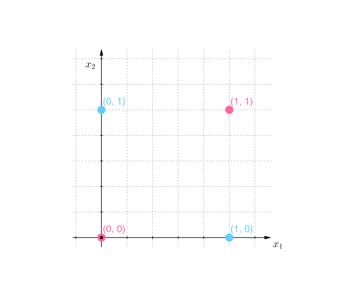
We can see from this image that there is no way to draw a line that separates the two classes. Thus, the perceptron algorithm would fail here, but a human would easily be able to see the rule that separates the two classes. The problem here is that the rule is not a linear divider.

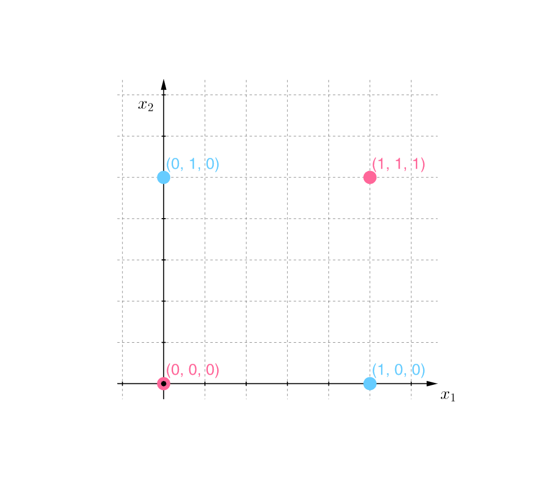
However, if we change our perspective on the problem, then a linear boundary becomes available. To see how this is done, note that the image shown appears to be two-dimensional.

If we instead view it as a plane in three dimensions \(\left( \mathbb{R}^3 \right)\), by adding a third coordinate, \(x_3\):

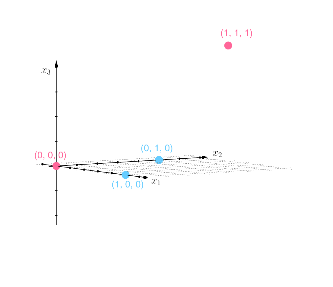
and rotate our view of the space like so:

we can see that a linear divider is indeed possible; one such divider is the plane defined by \(2x_3 - x_1 - x_2 + \tfrac{1}{2} = 0\):

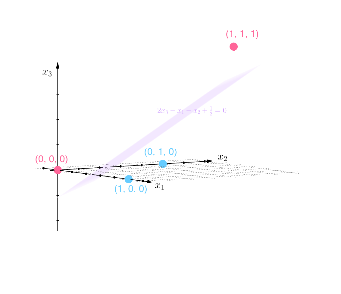
The adding of a third coordinate to our samples is akin to adding a new feature to the feature vectors comprising our inputs. This process of adding features is known as feature engineering, and is an essential tool in improving the performance of classifiers (and machine learning models in general). Furthermore, setting machine learning aside completely, the general technique of adding information that can change our perspective on a problem, is a great principle to apply to solving any problem in general!

References